Process NASA Earth Data
Analyze sea surface temperatures without downloading terabytes
Introduction#
NASA's Earth science repositories contain petabytes of climate and environmental data that traditionally require downloading before analysis—a slow and expensive process.
This example shows how to analyze sea surface temperature data directly in the cloud, examining temperature patterns in the Great Lakes region. By running your computation where the data lives, you'll eliminate hours of downloading time and drastically reduce costs.
The analysis processes 500GB of data in just 9 minutes instead of 6+ hours, at a fraction of the cost. You'll need the following packages:
pip install coiled earthaccess xarray numpy matplotlib
pip install coiled earthaccess xarray numpy matplotlib
Full code#
Run this code to analyze sea surface temperature variations. If you're new to Coiled, this will run for free on our account.
import coiled
import os
import tempfile
import earthaccess
import numpy as np
import xarray as xr
import matplotlib.pyplot as plt

# Step 1: Set up Earthdata authentication
# You'll need a free NASA Earthdata account (https://urs.earthdata.nasa.gov/)
earthaccess.login()

# Step 2: Find the dataset files we want to analyze
granules = earthaccess.search_data(
    short_name="MUR-JPL-L4-GLOB-v4.1",  # Sea Surface Temperature dataset
    temporal=("2020-01-01", "2021-12-31"),  # Two years of data
)

# Step 3: Create a function to process each data file
@coiled.function(
    region="us-west-2",                  # Run in the same region as data
    environ=earthaccess.auth_environ(),  # Forward Earthdata auth to cloud VMs
    spot_policy="spot_with_fallback",    # Use spot instances when available
    arm=True,                            # Use ARM-based instances
    cpu=1,                               # Use single-core instances
)
def process(granule):
    """Process a single data granule to extract Great Lakes temperature data"""
    results = []
    with tempfile.TemporaryDirectory() as tmpdir:
        files = earthaccess.download(granule, tmpdir)
        for file in files:
            ds = xr.open_dataset(os.path.join(tmpdir, file))
            # Select Great Lakes region by longitude/latitude
            ds = ds.sel(lon=slice(-93, -76), lat=slice(41, 49))
            # Filter for water temperature (exclude ice-covered areas)
            cond = (ds.sea_ice_fraction < 0.15) | np.isnan(ds.sea_ice_fraction)
            result = ds.analysed_sst.where(cond)
            results.append(result)
    return xr.concat(results, dim="time")

# Step 4: Run processing across all files in parallel
results = process.map(granules)

# Step 5: Combine results and visualize
ds = xr.concat(results, dim="time")

# Calculate temperature standard deviation across time
plt.figure(figsize=(14, 6))
std_temp = ds.std("time")
std_temp.plot(x="lon", y="lat", cmap="viridis")
plt.title("Standard Deviation of Sea Surface Temperature (2020-2021)")
plt.xlabel("Longitude")
plt.ylabel("Latitude")
plt.savefig("great_lakes_sst_variation.png")
plt.show()
After running this code, we'll explore what happened and why cloud-based processing is transformative for Earth science data analysis.
The Problem#
NASA's Earth Observing System Data and Information System (EOSDIS) hosts petabytes of Earth science data—including measurements of sea surface temperatures, precipitation, atmospheric composition, and more. These datasets are invaluable for climate research, environmental monitoring, and disaster response.
The challenge? The Multi-scale Ultra-high Resolution (MUR) Sea Surface Temperature dataset we're using is about 500GB for the time period we selected. Downloading this much data would:
- Take 6+ hours on a typical internet connection
- Cost approximately $25 in AWS data egress fees
- Require sufficient local storage space
- Demand substantial memory for processing
Scientists often find themselves spending more time managing data than analyzing it. This problem is only growing as datasets increase in size and resolution.
Cloud-Native Data Processing#
Instead of downloading data to our laptop, we'll bring our computation to the data using Coiled. This cloud-native approach offers massive advantages:
# Define a function to process data files
@coiled.function(
    region="us-west-2",                  # Run in the same region as data
    environ=earthaccess.auth_environ(),  # Forward Earthdata auth to cloud VMs
    spot_policy="spot_with_fallback",    # Use spot instances when available
    arm=True,                            # Use ARM-based instances
    cpu=1,                               # Use single-core instances
)
def process(granule):
    # Function body stays the same as it would locally
    ...
The @coiled.function decorator transforms our local function into one that runs in the cloud.
Key cloud configuration details:
- Region: We run in
us-west-2because that's where NASA stores this dataset - Authentication: We forward our Earthdata credentials to the cloud workers
- Cost optimization: We use spot instances, ARM processors, and right-sized VMs
Parallelizing the Workload#
The real power comes when we run our function across many files in parallel:
# Traditional approach - slow serial processing
for granule in granules:
    result = process(granule)
    results.append(result)
# Traditional approach - slow serial processing
for granule in granules:
    result = process(granule)
    results.append(result)
# Cloud approach - fast parallel processing
results = process.map(granules)
# Cloud approach - fast parallel processing
results = process.map(granules)
With a single line change, we're now processing hundreds of files simultaneously. Coiled automatically:
- Spins up the right number of cloud VMs
- Distributes the workload
- Gathers the results
- Cleans up resources when done

Analyzing the Results#
Once processing is complete, we combine the results from all files and calculate the standard deviation of sea surface temperatures over time:
# Combine all processed data
ds = xr.concat(results, dim="time")

# Calculate and plot temperature variation
plt.figure(figsize=(14, 6))
std_temp = ds.std("time")
std_temp.plot(x="lon", y="lat", cmap="viridis")
# Combine all processed data
ds = xr.concat(results, dim="time")

# Calculate and plot temperature variation
plt.figure(figsize=(14, 6))
std_temp = ds.std("time")
std_temp.plot(x="lon", y="lat", cmap="viridis")
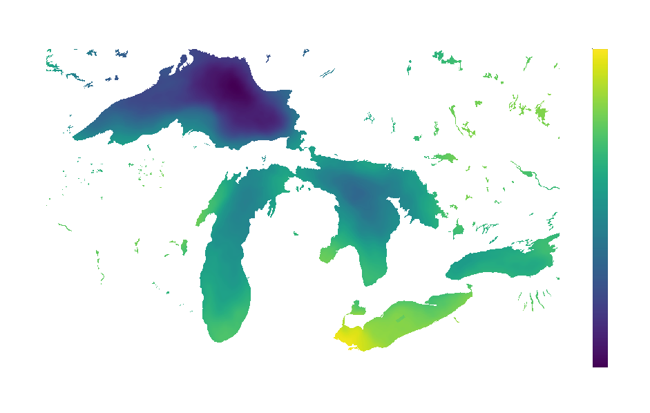
The resulting visualization reveals fascinating patterns in temperature variability across the Great Lakes:
Areas with higher standard deviation (brighter colors) indicate locations where temperature fluctuates more dramatically throughout the year.
Results#
Our cloud-native approach delivered impressive performance improvements:
The dramatic improvements come from:
- Data-proximate computing: Running code where the data is stored
- Massive parallelization: Processing many files simultaneously
- Cost optimization: Using the right instances for the job
Next Steps#
Here are some ways you could extend this example:
- Analyze different NASA Earth datasets like atmospheric composition or precipitation
- Compare sea surface temperatures across different regions or time periods
- Identify correlations between sea surface temperature and other climate variables
- Implement more complex analyses like anomaly detection or trend analysis
- Scale to even larger datasets by adjusting the cluster size
You could also try processing different NASA datasets available in the cloud:
# Search for aerosol optical depth data
granules = earthaccess.search_data(
    short_name="MOD04_L2",
    temporal=("2020-01-01", "2020-01-31")
)
# Search for aerosol optical depth data
granules = earthaccess.search_data(
    short_name="MOD04_L2",
    temporal=("2020-01-01", "2020-01-31")
)
Get started
Know Python? Come use the cloud. Your first $25 of usage per month is on us.
$ pip install coiled
$ coiled quickstart

Grant cloud access? (Y/n): Y

... Configuring  ...

You're ready to go. 🎉
$ pip install coiled
$ coiled quickstart
Grant cloud access? (Y/n): Y
... Configuring ...
You're ready to go. 🎉