Process Geospatial Data with Xarray
Calculate soil saturation for every US county in the cloud
Introduction#
Analyzing large-scale geospatial datasets presents significant computational challenges. This example shows how to use Xarray, Dask, and Coiled to process terabyte-scale hydrological data in the cloud, producing county-level soil saturation metrics across the entire United States.
The calculation processes 6TB of National Water Model data for the year 2020 in about 8 minutes, costing around $0.77. This same task would take days locally, if it ran at all. You can run it right now with these packages:
pip install coiled dask xarray flox rioxarray zarr s3fs geopandas matplotlib
pip install coiled dask xarray flox rioxarray zarr s3fs geopandas matplotlib
Full code#
Run this code to analyze soil saturation across all US counties. If you're new to Coiled, this will run for free on our account.
import coiled
import fsspec
import numpy as np
import rioxarray
import xarray as xr
import geopandas as gpd
import matplotlib.pyplot as plt
from flox.xarray import xarray_reduce

# Create a Coiled cluster in the same region as our data
cluster = coiled.Cluster(
    name="xarray-nwm",
    region="us-east-1",
    n_workers=10,
    worker_vm_types="r6g.xlarge",
)
client = cluster.get_client()

# Load the dataset and filter to just 2020
ds = xr.open_zarr(
    fsspec.get_mapper("s3://noaa-nwm-retrospective-2-1-zarr-pds/rtout.zarr", anon=True),
    consolidated=True,
    chunks={"time": 200, "x": 200, "y": 200}
)
ds = ds.sel(time=slice("2020-01-01", "2020-12-31"))

# Load US counties shapefile
counties = gpd.read_file("https://www2.census.gov/geo/tiger/GENZ2018/shp/cb_2018_us_county_500k.zip")
counties = counties.to_crs(ds.rio.crs)

# Set spatial dimensions
ds = ds.rio.write_crs(ds.crs)
ds = ds.rio.set_spatial_dims(x_dim="x", y_dim="y")

# Extract the soil saturation variable
zwattablrt = ds.ZWATTABLRT

# Calculate county-level means
result = xarray_reduce(
    zwattablrt,
    counties.geometry,
    func="mean"
)

# Plot the results
fig, ax = plt.subplots(1, 1, figsize=(12, 8))
counties.plot(ax=ax, color="lightgrey", edgecolor="grey", linewidth=0.3)
counties.plot(
    column=result.values,
    ax=ax,
    legend=True,
    cmap="viridis_r",
    vmin=0,
    vmax=5,
    edgecolor="grey",
    linewidth=0.3,
)
ax.set_title("Mean Depth to Soil Saturation (m) by US County - 2020")
plt.tight_layout()
plt.show()
After you've run this code, we'll explore what makes this approach so efficient compared to traditional methods.
The Problem#
The National Water Model (NWM) is a hydrological modeling framework that simulates streamflow, soil moisture, and other water-related variables across the entire United States. Government agencies, researchers, and water resource managers use this data to make critical decisions about:
- Drought monitoring and prediction
- Flood forecasting
- Agricultural planning
- Water supply management
- Climate change impact assessment
The NWM data presents several significant computational challenges:
- Massive scale: The full dataset spans decades and contains petabytes of information
- High resolution: Data at 250m spatial resolution with measurements every 3 hours
- Complex structure: Multi-dimensional arrays with spatial, temporal, and variable dimensions
- Integration challenge: Needs to be analyzed with respect to political boundaries (counties)
For our analysis of just one year (2020), we're working with:
- 6 terabytes of data
- 2,920 time steps (measurements every 3 hours for 365 days)
- Billions of individual grid cells across the continental US (250m resolution)
Attempting to download and process this data locally would be impractical:
- Download time: 12-24 hours with a fast connection
- Storage requirements: 6TB of free space
- Memory needs: Far exceeds most laptops/desktops
- Processing time: Days or weeks on a single machine
Setting Up Cloud Infrastructure#
The solution is to bring our computation to the data using Coiled's distributed computing capabilities. We'll set up a cluster in the same AWS region where the NWM data is stored:
# Create a Coiled cluster in AWS us-east-1 with ARM-based instances
cluster = coiled.Cluster(
    name="xarray-nwm",
    region="us-east-1",
    n_workers=10,
    worker_vm_types="r6g.xlarge",
)
client = cluster.get_client()
# Create a Coiled cluster in AWS us-east-1 with ARM-based instances
cluster = coiled.Cluster(
    name="xarray-nwm",
    region="us-east-1",
    n_workers=10,
    worker_vm_types="r6g.xlarge",
)
client = cluster.get_client()
We select r6g.xlarge instances which are:
- ARM-based (cheaper than x86)
- Memory-optimized (important for data processing)
- Appropriately sized for this workload
Loading and Filtering the Data#
Instead of downloading the data, we access it directly in the cloud:
# Load the NWM dataset from S3 and filter to 2020
ds = xr.open_zarr(
    fsspec.get_mapper("s3://noaa-nwm-retrospective-2-1-zarr-pds/rtout.zarr", anon=True),
    consolidated=True,
    chunks={"time": 200, "x": 200, "y": 200}
)
ds = ds.sel(time=slice("2020-01-01", "2020-12-31"))
# Load the NWM dataset from S3 and filter to 2020
ds = xr.open_zarr(
    fsspec.get_mapper("s3://noaa-nwm-retrospective-2-1-zarr-pds/rtout.zarr", anon=True),
    consolidated=True,
    chunks={"time": 200, "x": 200, "y": 200}
)
ds = ds.sel(time=slice("2020-01-01", "2020-12-31"))
Proper chunking is important for performance. We use moderate chunk sizes that will allow our computation to run efficiently across the workers.
Spatial Analysis with Xarray#
The heart of our analysis combines the NWM data with county boundaries to calculate average soil saturation levels for each US county:
# Load county boundaries and ensure compatible projection
counties = gpd.read_file("https://www2.census.gov/geo/tiger/GENZ2018/shp/cb_2018_us_county_500k.zip")
counties = counties.to_crs(ds.rio.crs)

# Prepare the dataset for spatial operations
ds = ds.rio.write_crs(ds.crs)
ds = ds.rio.set_spatial_dims(x_dim="x", y_dim="y")

# Extract soil saturation and calculate county-level means
zwattablrt = ds.ZWATTABLRT
result = xarray_reduce(
    zwattablrt,
    counties.geometry,
    func="mean"
)
This is where the distributed power of Xarray and Dask becomes critical:
- The computation is automatically divided across our 10 workers
- Each worker processes different chunks of the data in parallel
- Results are aggregated across all counties (3,000+ geometries)
- The entire operation runs without loading the full dataset into memory
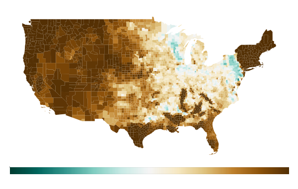
Results#
The cloud-based approach delivered remarkable performance improvements:
The final result is a comprehensive map showing soil saturation levels across all US counties:
/>
The performance improvements came from:
- Using appropriate chunk sizes for the computation
- Selecting memory-optimized ARM instances for better price/performance
- Running close to the data to avoid egress costs
- Utilizing Dask for distributed processing
Next Steps#
Here are some ways you could extend this example:
- Temporal analysis: Track how soil saturation changes across seasons or compare multiple years
- Correlation studies: Combine with precipitation or temperature data to identify relationships
- Extreme event focus: Zoom in on specific drought or flood events during 2020
- Different variables: Analyze other NWM outputs like streamflow, evapotranspiration, or snow water equivalent
- Alternative boundaries: Use watersheds, climate regions, or agricultural zones instead of counties
- Performance tuning: Experiment with different worker counts and chunk sizes to optimize for your specific analysis
You could also apply this pattern to other large geospatial datasets:
# Example: NASA CMIP6 climate projections
ds = xr.open_zarr(
    fsspec.get_mapper("s3://cmip6-pds/CMIP6/ScenarioMIP/...", anon=True),
    chunks={"time": 365, "lat": 100, "lon": 100}
)

# Example: NOAA GOES satellite imagery
ds = xr.open_zarr(
    fsspec.get_mapper("s3://noaa-goes16/ABI-L1b-RadC/...", anon=True),
    chunks={"time": 24, "y": 1000, "x": 1000}
)
Get started
Know Python? Come use the cloud. Your first $25 of usage per month is on us.
$ pip install coiled
$ coiled quickstart

Grant cloud access? (Y/n): Y

... Configuring  ...

You're ready to go. 🎉
$ pip install coiled
$ coiled quickstart
Grant cloud access? (Y/n): Y
... Configuring ...
You're ready to go. 🎉